measuring real-world ai progress
Every time a new model drops, headline benchmark scores flood my feed. But for anyone running these systems in production, those numbers are becoming increasingly hard to compare.
To bridge theory and practice, the ecosystem needs better reporting:
-
Model providers: report benchmark performance against test-time compute. We all see the Pareto curves on launch day. But if Model A uses 10x the inference budget of Model B — more reasoning tokens, longer trajectories, or extra retries — it isn't an apples-to-apples comparison.
At minimum, give us controlled comparisons at equivalent test-time compute; better still, publish the full TTC curve. Test-time scaling directly impacts inference cost per task, which is a core metric for production operators. A simple plot like Fig. 1 from Charlie Snell, et al will do (see below).
-
Harness providers: publish ablations.
When an eval framework shows an incumbent model beating a newer release on real-world tasks, show us performance under both a naive/open harness and an 'optimized' harness for the relevant domain.
'Custom' harnesses encode assumptions about past model failure modes. Planning loops, critics, and strict tool constraints were often built to patch the weaknesses of last-gen model(s). A next-gen model might no longer need that scaffolding; worse, the harness (optimized for model n-1) might actively restrict performance gains on model n. Without ablations, we can't separate model capability from harness compatibility.
AI Leaders: understanding these interactions isn't optional anymore. You can't credibly drive an enterprise AI strategy without mapping the relationship between raw model capability, test-time compute and harness design (table stakes).
Why? Because it directly impacts your unit economics. 💰
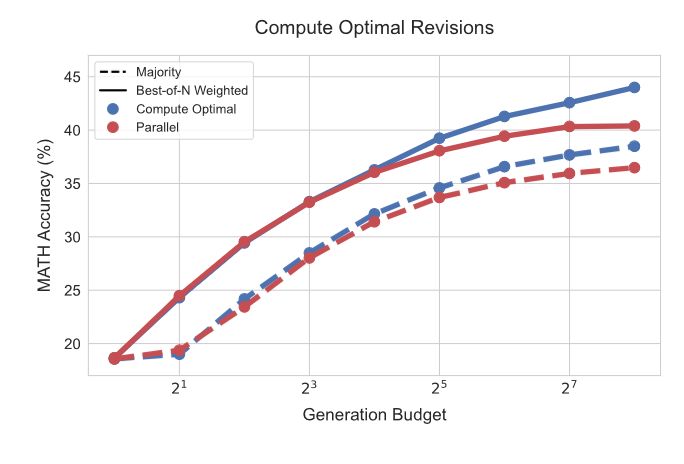
Fig. 1 from Snell, Lee, Xu, Kumar (2024). 'Scaling LLM Test-Time Compute Optimally can be More Effective than Scaling Model Parameters'.